Portfolio
My classwork from bimm143
Class08
Samuel Fisher (A18131929)
Save your input data file into your Project directory
fna.data <- “WisconsinCancer.csv”
Complete the following code to input the data and store as wisc.df
wisc.df <- ___(fna.data, row.names=1)
Exploratory Data Analysis
First we load the Wisconsin cancer dataset and prepare it for analysis.
fna.data <- "WisconsinCancer.csv"
wisc.df <- read.csv(fna.data, row.names=1)
head(wisc.df, 4)
         diagnosis radius_mean texture_mean perimeter_mean area_mean
842302           M       17.99        10.38         122.80    1001.0
842517           M       20.57        17.77         132.90    1326.0
84300903         M       19.69        21.25         130.00    1203.0
84348301         M       11.42        20.38          77.58     386.1
         smoothness_mean compactness_mean concavity_mean concave.points_mean
842302           0.11840          0.27760         0.3001             0.14710
842517           0.08474          0.07864         0.0869             0.07017
84300903         0.10960          0.15990         0.1974             0.12790
84348301         0.14250          0.28390         0.2414             0.10520
         symmetry_mean fractal_dimension_mean radius_se texture_se perimeter_se
842302          0.2419                0.07871    1.0950     0.9053        8.589
842517          0.1812                0.05667    0.5435     0.7339        3.398
84300903        0.2069                0.05999    0.7456     0.7869        4.585
84348301        0.2597                0.09744    0.4956     1.1560        3.445
         area_se smoothness_se compactness_se concavity_se concave.points_se
842302    153.40      0.006399        0.04904      0.05373           0.01587
842517     74.08      0.005225        0.01308      0.01860           0.01340
84300903   94.03      0.006150        0.04006      0.03832           0.02058
84348301   27.23      0.009110        0.07458      0.05661           0.01867
         symmetry_se fractal_dimension_se radius_worst texture_worst
842302       0.03003             0.006193        25.38         17.33
842517       0.01389             0.003532        24.99         23.41
84300903     0.02250             0.004571        23.57         25.53
84348301     0.05963             0.009208        14.91         26.50
         perimeter_worst area_worst smoothness_worst compactness_worst
842302            184.60     2019.0           0.1622            0.6656
842517            158.80     1956.0           0.1238            0.1866
84300903          152.50     1709.0           0.1444            0.4245
84348301           98.87      567.7           0.2098            0.8663
         concavity_worst concave.points_worst symmetry_worst
842302            0.7119               0.2654         0.4601
842517            0.2416               0.1860         0.2750
84300903          0.4504               0.2430         0.3613
84348301          0.6869               0.2575         0.6638
         fractal_dimension_worst
842302                   0.11890
842517                   0.08902
84300903                 0.08758
84348301                 0.17300
We remove the diagnosis column so unsupervised methods do not use the known labels.
wisc.data <- wisc.df[, -1]
Diagnosis Vector
We save the diagnosis column as a factor for later comparison and plotting.
diagnosis <- as.factor(wisc.df$diagnosis)
Q1 - Number of observations
We check how many observations (rows) are in the dataset.
nrow(wisc.data)
[1] 569
There are 569 observations in the dataset
Q2 - Number of malignant samples
We want to count how many samples are labeled malignant in the diagnosis vector.
table(diagnosis)
diagnosis
  B   M
357 212
212 observations are malignant
Q3 - Number of _mean features
We want to count how many variable names end with _mean.
length(grep("_mean$", colnames(wisc.data)))
[1] 10
10 variables names end with _mean
Principal Component Analysis
Check column means and standard deviations
colMeans(wisc.data)
            radius_mean            texture_mean          perimeter_mean
           1.412729e+01            1.928965e+01            9.196903e+01
              area_mean         smoothness_mean        compactness_mean
           6.548891e+02            9.636028e-02            1.043410e-01
         concavity_mean     concave.points_mean           symmetry_mean
           8.879932e-02            4.891915e-02            1.811619e-01
 fractal_dimension_mean               radius_se              texture_se
           6.279761e-02            4.051721e-01            1.216853e+00
           perimeter_se                 area_se           smoothness_se
           2.866059e+00            4.033708e+01            7.040979e-03
         compactness_se            concavity_se       concave.points_se
           2.547814e-02            3.189372e-02            1.179614e-02
            symmetry_se    fractal_dimension_se            radius_worst
           2.054230e-02            3.794904e-03            1.626919e+01
          texture_worst         perimeter_worst              area_worst
           2.567722e+01            1.072612e+02            8.805831e+02
       smoothness_worst       compactness_worst         concavity_worst
           1.323686e-01            2.542650e-01            2.721885e-01
   concave.points_worst          symmetry_worst fractal_dimension_worst
           1.146062e-01            2.900756e-01            8.394582e-02
apply(wisc.data, 2, sd)
            radius_mean            texture_mean          perimeter_mean
           3.524049e+00            4.301036e+00            2.429898e+01
              area_mean         smoothness_mean        compactness_mean
           3.519141e+02            1.406413e-02            5.281276e-02
         concavity_mean     concave.points_mean           symmetry_mean
           7.971981e-02            3.880284e-02            2.741428e-02
 fractal_dimension_mean               radius_se              texture_se
           7.060363e-03            2.773127e-01            5.516484e-01
           perimeter_se                 area_se           smoothness_se
           2.021855e+00            4.549101e+01            3.002518e-03
         compactness_se            concavity_se       concave.points_se
           1.790818e-02            3.018606e-02            6.170285e-03
            symmetry_se    fractal_dimension_se            radius_worst
           8.266372e-03            2.646071e-03            4.833242e+00
          texture_worst         perimeter_worst              area_worst
           6.146258e+00            3.360254e+01            5.693570e+02
       smoothness_worst       compactness_worst         concavity_worst
           2.283243e-02            1.573365e-01            2.086243e-01
   concave.points_worst          symmetry_worst fractal_dimension_worst
           6.573234e-02            6.186747e-02            1.806127e-02
The variables have very different standard deviations, so scaling is required before performing PCA.
PCA Model
Perform PCA on wisc.data by completing the following code
wisc.pr <- prcomp(wisc.data, scale = TRUE)
We want to look over the PCA summary to see how much variance of each principal component
summary(wisc.pr)
Importance of components:
                          PC1    PC2     PC3     PC4     PC5     PC6     PC7
Standard deviation     3.6444 2.3857 1.67867 1.40735 1.28403 1.09880 0.82172
Proportion of Variance 0.4427 0.1897 0.09393 0.06602 0.05496 0.04025 0.02251
Cumulative Proportion  0.4427 0.6324 0.72636 0.79239 0.84734 0.88759 0.91010
                           PC8    PC9    PC10   PC11    PC12    PC13    PC14
Standard deviation     0.69037 0.6457 0.59219 0.5421 0.51104 0.49128 0.39624
Proportion of Variance 0.01589 0.0139 0.01169 0.0098 0.00871 0.00805 0.00523
Cumulative Proportion  0.92598 0.9399 0.95157 0.9614 0.97007 0.97812 0.98335
                          PC15    PC16    PC17    PC18    PC19    PC20   PC21
Standard deviation     0.30681 0.28260 0.24372 0.22939 0.22244 0.17652 0.1731
Proportion of Variance 0.00314 0.00266 0.00198 0.00175 0.00165 0.00104 0.0010
Cumulative Proportion  0.98649 0.98915 0.99113 0.99288 0.99453 0.99557 0.9966
                          PC22    PC23   PC24    PC25    PC26    PC27    PC28
Standard deviation     0.16565 0.15602 0.1344 0.12442 0.09043 0.08307 0.03987
Proportion of Variance 0.00091 0.00081 0.0006 0.00052 0.00027 0.00023 0.00005
Cumulative Proportion  0.99749 0.99830 0.9989 0.99942 0.99969 0.99992 0.99997
                          PC29    PC30
Standard deviation     0.02736 0.01153
Proportion of Variance 0.00002 0.00000
Cumulative Proportion  1.00000 1.00000
Q4 - Variance found by PC1
Proportion of Variance — PC1 = 0.4427, therefore PC1 captures 44.27% of the total variance.
Q5 - PCs needed for 70% variance
PC1 = 0.4427 PC2 = 0.6324 PC3 = 0.72636 ← first value greater than or equal to 0.70
Three principal components are needed to explain at least 70% of the variance.
Q6 - PCs needed for 90% variance
PC6 = 0.88759 PC7 = 0.91010 ← first value greater than or equal to 0.90 Seven principal components are needed to explain at least 90% of the variance.
Interpreting PCA Results
We want to create a PCA biplot to visualize both sample scores and feature loadings.
biplot(wisc.pr)
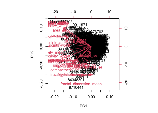
Q7 - Biplot Interpretation
The biplot is incredibly difficult to interpret because it is chaotic and with many things overlapping. The row labels are all over the figure, making patterns and group separation hard to see and understand.
PC1 vs PC2 Plot
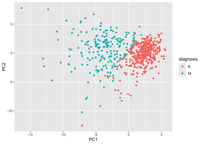
Scatter plot observations by components 1 and 2
library(ggplot2)
ggplot(wisc.pr$x) +
  aes(PC1, PC2, col = diagnosis) +
  geom_point()
Q8 - Compare plots of PC1 vs PC2 to plot of PC1 vs PC3
ggplot(wisc.pr$x) +
  aes(PC1, PC3, col = diagnosis) +
  geom_point()
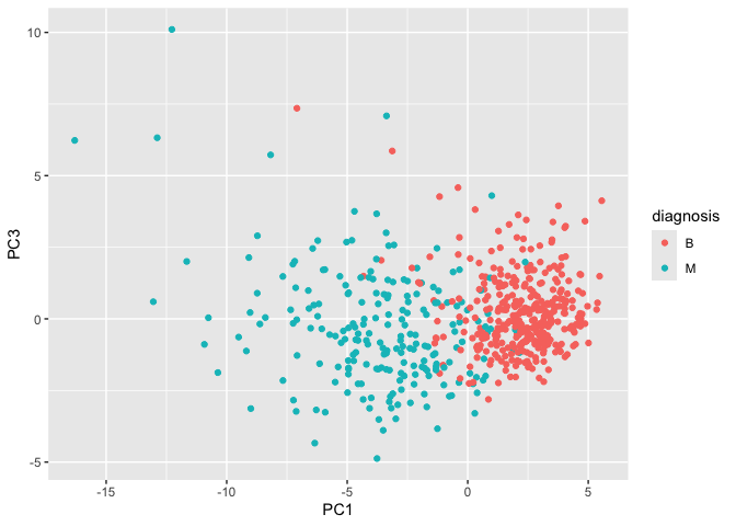
PC1 vs PC3 Plot
The PC1 vs PC2 plot has a clearer separation between M and B samples than the PC1 vs PC3 plot. This shows that PC2 captures more class-separating structure than PC3. PC1 seems to drive most of the separation overall, while later components add less discriminatory power.
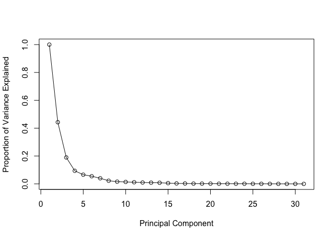
Variance Explained
Calculate variance of each component
pr.var <- wisc.pr$sdev^2
head(pr.var)
[1] 13.281608 5.691355 2.817949 1.980640 1.648731 1.207357
pve <- pr.var / sum(pr.var)
plot(c(1,pve), xlab = "Principal Component",
ylab = "Proportion of Variance Explained",
ylim = c(0, 1), type = "o")
Alternative scree plot of the same data, note data driven y-axis
barplot(pve, ylab = "Percent of Variance Explained",
names.arg=paste0("PC",1:length(pve)), las=2, axes = FALSE)
axis(2, at=pve, labels=round(pve,2)*100 )
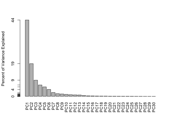
Q9 — Plot Interpretation
wisc.pr$rotation["concave.points_mean", 1]
[1] -0.2608538
sort(wisc.pr$rotation[,1], decreasing=TRUE)[1:5]
         smoothness_se             texture_se            symmetry_se
           -0.01453145            -0.01742803            -0.04249842
fractal_dimension_mean   fractal_dimension_se
           -0.06436335            -0.10256832
sort(abs(wisc.pr$rotation[,1]), decreasing=TRUE)[1:5]
 concave.points_mean       concavity_mean concave.points_worst
           0.2608538            0.2584005            0.2508860
    compactness_mean      perimeter_worst
           0.2392854            0.2366397
The loading value for concave.points_mean in PC1 is 0.2608538. There are no features with a larger absolute loading than this one. It is the largest contributor to PC1 (with concavity_mean and concave.points_worst being slightly smaller but similar).
Hierarchical Clustering
data.scaled <- scale(wisc.data)
data.dist <- dist(data.scaled)
Perform hierarchical clustering using complete linkage and plot
wisc.hclust <- hclust(data.dist, method = "complete")
plot(wisc.hclust)
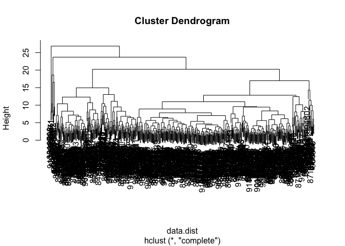
Q10
plot(wisc.hclust)
abline(h = 15, col="red", lty=2)
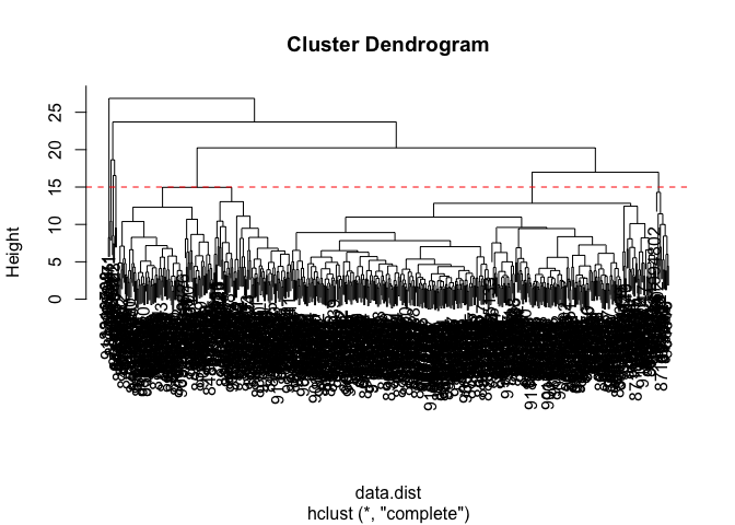
The height at which the clustering model has 4 clusters is approximately 15.
wisc.clusters <- cutree(wisc.hclust, k = 4)
table(wisc.clusters, diagnosis)
             diagnosis
wisc.clusters   B   M
            1  12 165
            2   2   5
            3 343  40
            4   0   2
Q12
Ward.D2 gives the best results because it creates the cleanest and most balanced cluster separation while minimizing cluster variance within, which fits this dataset well.
Clustering on PCA Results
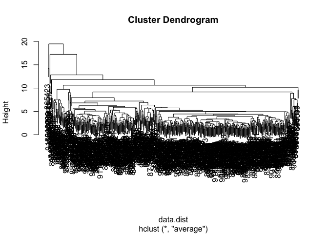
We will do the hierarchical clustering again but using average linkage to compare results.
wisc.hclust.avg <- hclust(data.dist, method = "average")
plot(wisc.hclust.avg)
wisc.clusters.avg <- cutree(wisc.hclust.avg, k = 2)
table(wisc.clusters.avg, diagnosis)
                 diagnosis
wisc.clusters.avg   B   M
                1 357 209
                2   0   3
Average Linkage Cluster Comparison
Using average linkage makes a similar result to complete linkage. The clusters still don’t align perfectly with diagnosis labels. This shows that hierarchical clustering w/o labels doesn’t perfectly separate B and M samples.
Clustering on PCA Scores
Hierarchical clustering on PCA scores (first 7 PCs)
pc.dist <- dist(wisc.pr$x[,1:7])
wisc.pr.hclust <- hclust(dist(wisc.pr$x[,1:7]), method = "ward.D2")
plot(wisc.pr.hclust)
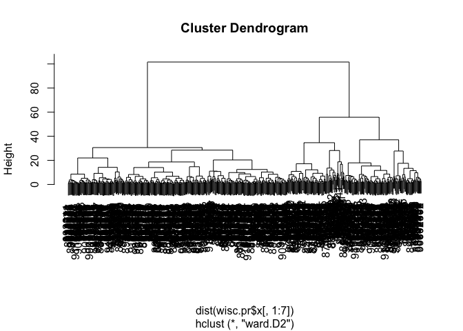
grps <- cutree(wisc.pr.hclust, k=2)
table(grps)
grps
  1   2
216 353
table(grps, diagnosis)
    diagnosis
grps   B   M
   1  28 188
   2 329  24
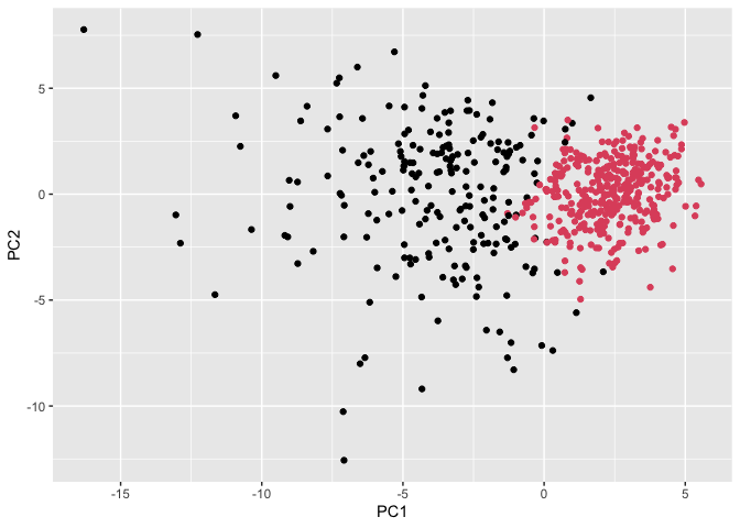
ggplot(wisc.pr$x) +
aes(PC1, PC2) +
geom_point(col=grps)
Use the distance along the first 7 PCs for clustering i.e. wisc.pr$x[, 1:7]
wisc.pr.hclust <- hclust(dist(wisc.pr$x[,1:7]), method="ward.D2")
wisc.pr.hclust.clusters <- cutree(wisc.pr.hclust, k=2)
Q13
Compare to actual diagnoses
table(wisc.pr.hclust.clusters, diagnosis)
                       diagnosis
wisc.pr.hclust.clusters   B   M
                      1  28 188
                      2 329  24
It separates pretty well, with 52 total misclassified. 28 Benign mixed into the mostly malignant cluster plus 24 malignant mixed into the mostly-benign cluster.
Q14
table(wisc.clusters, diagnosis)
             diagnosis
wisc.clusters   B   M
            1  12 165
            2   2   5
            3 343  40
            4   0   2
Clustering on the PCA transformed data separates the diagnoses better than clustering on the original features. The PCA based model generates two better clusters that have less mixed benign/malignant cases. The original data clustering spreads samples across more mixed clusters.
Prediction
#url <- "new_samples.csv"
url <- "https://tinyurl.com/new-samples-CSV"
new <- read.csv(url)
npc <- predict(wisc.pr, newdata=new)
npc
           PC1       PC2        PC3        PC4       PC5        PC6        PC7
[1,]  2.576616 -3.135913  1.3990492 -0.7631950  2.781648 -0.8150185 -0.3959098
[2,] -4.754928 -3.009033 -0.1660946 -0.6052952 -1.140698 -1.2189945  0.8193031
            PC8       PC9       PC10      PC11      PC12      PC13     PC14
[1,] -0.2307350 0.1029569 -0.9272861 0.3411457  0.375921 0.1610764 1.187882
[2,] -0.3307423 0.5281896 -0.4855301 0.7173233 -1.185917 0.5893856 0.303029
          PC15       PC16        PC17        PC18        PC19       PC20
[1,] 0.3216974 -0.1743616 -0.07875393 -0.11207028 -0.08802955 -0.2495216
[2,] 0.1299153  0.1448061 -0.40509706  0.06565549  0.25591230 -0.4289500
           PC21       PC22       PC23       PC24        PC25         PC26
[1,]  0.1228233 0.09358453 0.08347651  0.1223396  0.02124121  0.078884581
[2,] -0.1224776 0.01732146 0.06316631 -0.2338618 -0.20755948 -0.009833238
             PC27        PC28         PC29         PC30
[1,]  0.220199544 -0.02946023 -0.015620933  0.005269029
[2,] -0.001134152  0.09638361  0.002795349 -0.019015820
plot(wisc.pr$x[,1:2], col=grps)
points(npc[,1], npc[,2], col="blue", pch=16, cex=3)
text(npc[,1], npc[,2], c(1,2), col="white")
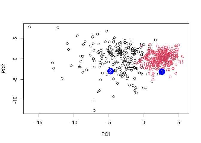
Q16
Patient 1 should be prioritized for a follow up because it falls within the malignant like cluster.Patient 2 groups with the benign like cluster.