Portfolio
My classwork from bimm143
Class 14
Samuel Fisher (A18131929)
Section 1: Differential Expression Analysis
library(DESeq2)
Loading required package: S4Vectors

Loading required package: stats4

Loading required package: BiocGenerics

Loading required package: generics


Attaching package: 'generics'

The following objects are masked from 'package:base':

    as.difftime, as.factor, as.ordered, intersect, is.element, setdiff,
    setequal, union


Attaching package: 'BiocGenerics'

The following objects are masked from 'package:stats':

    IQR, mad, sd, var, xtabs

The following objects are masked from 'package:base':

    anyDuplicated, aperm, append, as.data.frame, basename, cbind,
    colnames, dirname, do.call, duplicated, eval, evalq, Filter, Find,
    get, grep, grepl, is.unsorted, lapply, Map, mapply, match, mget,
    order, paste, pmax, pmax.int, pmin, pmin.int, Position, rank,
    rbind, Reduce, rownames, sapply, saveRDS, table, tapply, unique,
    unsplit, which.max, which.min


Attaching package: 'S4Vectors'

The following object is masked from 'package:utils':

    findMatches

The following objects are masked from 'package:base':

    expand.grid, I, unname

Loading required package: IRanges

Loading required package: GenomicRanges

Loading required package: Seqinfo

Loading required package: SummarizedExperiment

Loading required package: MatrixGenerics

Loading required package: matrixStats


Attaching package: 'MatrixGenerics'

The following objects are masked from 'package:matrixStats':

    colAlls, colAnyNAs, colAnys, colAvgsPerRowSet, colCollapse,
    colCounts, colCummaxs, colCummins, colCumprods, colCumsums,
    colDiffs, colIQRDiffs, colIQRs, colLogSumExps, colMadDiffs,
    colMads, colMaxs, colMeans2, colMedians, colMins, colOrderStats,
    colProds, colQuantiles, colRanges, colRanks, colSdDiffs, colSds,
    colSums2, colTabulates, colVarDiffs, colVars, colWeightedMads,
    colWeightedMeans, colWeightedMedians, colWeightedSds,
    colWeightedVars, rowAlls, rowAnyNAs, rowAnys, rowAvgsPerColSet,
    rowCollapse, rowCounts, rowCummaxs, rowCummins, rowCumprods,
    rowCumsums, rowDiffs, rowIQRDiffs, rowIQRs, rowLogSumExps,
    rowMadDiffs, rowMads, rowMaxs, rowMeans2, rowMedians, rowMins,
    rowOrderStats, rowProds, rowQuantiles, rowRanges, rowRanks,
    rowSdDiffs, rowSds, rowSums2, rowTabulates, rowVarDiffs, rowVars,
    rowWeightedMads, rowWeightedMeans, rowWeightedMedians,
    rowWeightedSds, rowWeightedVars

Loading required package: Biobase

Welcome to Bioconductor

    Vignettes contain introductory material; view with
    'browseVignettes()'. To cite Bioconductor, see
    'citation("Biobase")', and for packages 'citation("pkgname")'.


Attaching package: 'Biobase'

The following object is masked from 'package:MatrixGenerics':

    rowMedians

The following objects are masked from 'package:matrixStats':

    anyMissing, rowMedians
metaFile  <- "GSE37704_metadata.csv"
countFile <- "GSE37704_featurecounts.csv"

# Import metadata and take a peek
colData <- read.csv(metaFile, row.names = 1)
head(colData)
              condition
SRR493366 control_sirna
SRR493367 control_sirna
SRR493368 control_sirna
SRR493369      hoxa1_kd
SRR493370      hoxa1_kd
SRR493371      hoxa1_kd
# Import countdata
countData <- read.csv(countFile, row.names = 1)
head(countData)
                length SRR493366 SRR493367 SRR493368 SRR493369 SRR493370
ENSG00000186092    918         0         0         0         0         0
ENSG00000279928    718         0         0         0         0         0
ENSG00000279457   1982        23        28        29        29        28
ENSG00000278566    939         0         0         0         0         0
ENSG00000273547    939         0         0         0         0         0
ENSG00000187634   3214       124       123       205       207       212
                SRR493371
ENSG00000186092         0
ENSG00000279928         0
ENSG00000279457        46
ENSG00000278566         0
ENSG00000273547         0
ENSG00000187634       258
Q. Complete the code below to remove the troublesome first column from countData
countData <- read.csv(countFile, row.names = 1)
countData <- as.matrix(countData[, -1])
head(countData)
                SRR493366 SRR493367 SRR493368 SRR493369 SRR493370 SRR493371
ENSG00000186092         0         0         0         0         0         0
ENSG00000279928         0         0         0         0         0         0
ENSG00000279457        23        28        29        29        28        46
ENSG00000278566         0         0         0         0         0         0
ENSG00000273547         0         0         0         0         0         0
ENSG00000187634       124       123       205       207       212       258
Q. Q. Complete the code below to filter countData to exclude genes (i.e. rows) where we have 0 read count across all samples (i.e. columns). Tip: What will rowSums() of countData return and how could you use it in this context?
# Filter count data where you have 0 read count across all samples.
countData = countData[rowSums(countData) > 0, ]
head(countData)
                SRR493366 SRR493367 SRR493368 SRR493369 SRR493370 SRR493371
ENSG00000279457        23        28        29        29        28        46
ENSG00000187634       124       123       205       207       212       258
ENSG00000188976      1637      1831      2383      1226      1326      1504
ENSG00000187961       120       153       180       236       255       357
ENSG00000187583        24        48        65        44        48        64
ENSG00000187642         4         9        16        14        16        16
Running DESeq2
dds = DESeqDataSetFromMatrix(countData = countData,
                             colData   = colData,
                             design    = ~condition)
Warning in DESeqDataSet(se, design = design, ignoreRank): some variables in
design formula are characters, converting to factors
dds = DESeq(dds)
estimating size factors

estimating dispersions

gene-wise dispersion estimates

mean-dispersion relationship

final dispersion estimates

fitting model and testing
dds
class: DESeqDataSet
dim: 15975 6
metadata(1): version
assays(4): counts mu H cooks
rownames(15975): ENSG00000279457 ENSG00000187634 ... ENSG00000276345
  ENSG00000271254
rowData names(22): baseMean baseVar ... deviance maxCooks
colnames(6): SRR493366 SRR493367 ... SRR493370 SRR493371
colData names(2): condition sizeFactor
res = results(dds)
res
log2 fold change (MLE): condition hoxa1 kd vs control sirna
Wald test p-value: condition hoxa1 kd vs control sirna
DataFrame with 15975 rows and 6 columns
                 baseMean log2FoldChange     lfcSE       stat      pvalue
                <numeric>      <numeric> <numeric>  <numeric>   <numeric>
ENSG00000279457   29.9136      0.1792571 0.3248216   0.551863 5.81042e-01
ENSG00000187634  183.2296      0.4264571 0.1402658   3.040350 2.36304e-03
ENSG00000188976 1651.1881     -0.6927205 0.0548465 -12.630158 1.43990e-36
ENSG00000187961  209.6379      0.7297556 0.1318599   5.534326 3.12428e-08
ENSG00000187583   47.2551      0.0405765 0.2718928   0.149237 8.81366e-01
...                   ...            ...       ...        ...         ...
ENSG00000273748  35.30265       0.674387  0.303666   2.220817 2.63633e-02
ENSG00000278817   2.42302      -0.388988  1.130394  -0.344117 7.30758e-01
ENSG00000278384   1.10180       0.332991  1.660261   0.200565 8.41039e-01
ENSG00000276345  73.64496      -0.356181  0.207716  -1.714752 8.63908e-02
ENSG00000271254 181.59590      -0.609667  0.141320  -4.314071 1.60276e-05
                       padj
                  <numeric>
ENSG00000279457 6.86555e-01
ENSG00000187634 5.15718e-03
ENSG00000188976 1.76549e-35
ENSG00000187961 1.13413e-07
ENSG00000187583 9.19031e-01
...                     ...
ENSG00000273748 4.79091e-02
ENSG00000278817 8.09772e-01
ENSG00000278384 8.92654e-01
ENSG00000276345 1.39762e-01
ENSG00000271254 4.53648e-05
Q. Call the summary() function on your results to get a sense of how many genes are up or down-regulated at the default 0.1 p-value cutoff.
summary(res)
out of 15975 with nonzero total read count
adjusted p-value < 0.1
LFC > 0 (up)       : 4349, 27%
LFC < 0 (down)     : 4396, 28%
outliers [1]       : 0, 0%
low counts [2]     : 1237, 7.7%
(mean count < 0)
[1] see 'cooksCutoff' argument of ?results
[2] see 'independentFiltering' argument of ?results
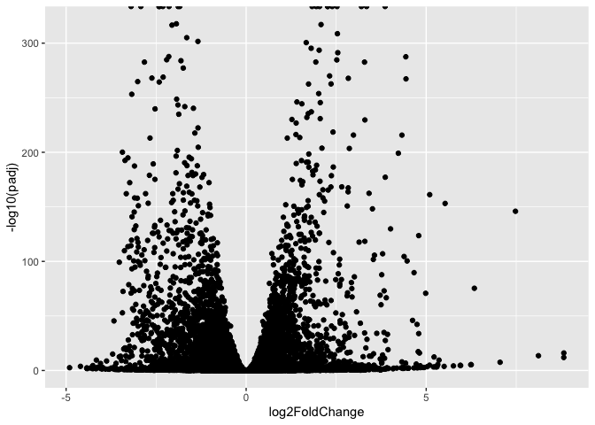
Volcano Plot
library(ggplot2)

ggplot(res) +
  aes(x = log2FoldChange,
      y = -log10(padj)) +
  geom_point()
Warning: Removed 1237 rows containing missing values or values outside the scale range
(`geom_point()`).
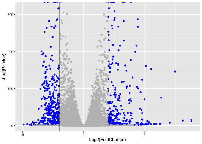
Q. Improve this plot by completing the below code, which adds color, axis labels and cutoff lines:
# Make a color vector for all genes
mycols <- rep("gray", nrow(res))

# Color blue the genes with fold change above 2
mycols[ abs(res$log2FoldChange) > 2 ] <- "blue"

# Color gray those with adjusted p-value more than 0.01
mycols[ res$padj > 0.01 ] <- "gray"

ggplot(res) +
  aes(x = log2FoldChange,
      y = -log10(padj)) +
  geom_point(color = mycols) +
  xlab("Log2(FoldChange)") +
  ylab("-Log(P-value)") +
  geom_vline(xintercept = c(-2,2)) +
  geom_hline(yintercept = -log10(0.01))
Warning: Removed 1237 rows containing missing values or values outside the scale range
(`geom_point()`).
Adding Gene Annotation
library("AnnotationDbi")
library("org.Hs.eg.db")
columns(org.Hs.eg.db)
 [1] "ACCNUM"       "ALIAS"        "ENSEMBL"      "ENSEMBLPROT"  "ENSEMBLTRANS"
 [6] "ENTREZID"     "ENZYME"       "EVIDENCE"     "EVIDENCEALL"  "GENENAME"
[11] "GENETYPE"     "GO"           "GOALL"        "IPI"          "MAP"
[16] "OMIM"         "ONTOLOGY"     "ONTOLOGYALL"  "PATH"         "PFAM"
[21] "PMID"         "PROSITE"      "REFSEQ"       "SYMBOL"       "UCSCKG"
[26] "UNIPROT"
res$symbol = mapIds(org.Hs.eg.db,
                    keys = row.names(res),
                    keytype = "ENSEMBL",
                    column = "SYMBOL",
                    multiVals = "first")
'select()' returned 1:many mapping between keys and columns
res$entrez = mapIds(org.Hs.eg.db,
                    keys = row.names(res),
                    keytype = "ENSEMBL",
                    column = "ENTREZID",
                    multiVals = "first")
'select()' returned 1:many mapping between keys and columns
res$name = mapIds(org.Hs.eg.db,
                  keys = row.names(res),
                  keytype = "ENSEMBL",
                  column = "GENENAME",
                  multiVals = "first")
'select()' returned 1:many mapping between keys and columns
head(res, 10)
log2 fold change (MLE): condition hoxa1 kd vs control sirna
Wald test p-value: condition hoxa1 kd vs control sirna
DataFrame with 10 rows and 9 columns
                   baseMean log2FoldChange     lfcSE       stat      pvalue
                  <numeric>      <numeric> <numeric>  <numeric>   <numeric>
ENSG00000279457   29.913579      0.1792571 0.3248216   0.551863 5.81042e-01
ENSG00000187634  183.229650      0.4264571 0.1402658   3.040350 2.36304e-03
ENSG00000188976 1651.188076     -0.6927205 0.0548465 -12.630158 1.43990e-36
ENSG00000187961  209.637938      0.7297556 0.1318599   5.534326 3.12428e-08
ENSG00000187583   47.255123      0.0405765 0.2718928   0.149237 8.81366e-01
ENSG00000187642   11.979750      0.5428105 0.5215598   1.040744 2.97994e-01
ENSG00000188290  108.922128      2.0570638 0.1969053  10.446970 1.51282e-25
ENSG00000187608  350.716868      0.2573837 0.1027266   2.505522 1.22271e-02
ENSG00000188157 9128.439422      0.3899088 0.0467163   8.346304 7.04321e-17
ENSG00000237330    0.158192      0.7859552 4.0804729   0.192614 8.47261e-01
                       padj      symbol      entrez                   name
                  <numeric> <character> <character>            <character>
ENSG00000279457 6.86555e-01          NA          NA                     NA
ENSG00000187634 5.15718e-03      SAMD11      148398 sterile alpha motif ..
ENSG00000188976 1.76549e-35       NOC2L       26155 NOC2 like nucleolar ..
ENSG00000187961 1.13413e-07      KLHL17      339451 kelch like family me..
ENSG00000187583 9.19031e-01     PLEKHN1       84069 pleckstrin homology ..
ENSG00000187642 4.03379e-01       PERM1       84808 PPARGC1 and ESRR ind..
ENSG00000188290 1.30538e-24        HES4       57801 hes family bHLH tran..
ENSG00000187608 2.37452e-02       ISG15        9636 ISG15 ubiquitin like..
ENSG00000188157 4.21963e-16        AGRN      375790                  agrin
ENSG00000237330          NA      RNF223      401934 ring finger protein ..
Q. Finally for this section let’s reorder these results by adjusted p-value and save them to a CSV file in your current project directory.
res = res[order(res$pvalue),]
write.csv(res, file="deseq_results.csv")
Section 2: Pathway analysis
library(pathview)
##############################################################################
Pathview is an open source software package distributed under GNU General
Public License version 3 (GPLv3). Details of GPLv3 is available at
http://www.gnu.org/licenses/gpl-3.0.html. Particullary, users are required to
formally cite the original Pathview paper (not just mention it) in publications
or products. For details, do citation("pathview") within R.

The pathview downloads and uses KEGG data. Non-academic uses may require a KEGG
license agreement (details at http://www.kegg.jp/kegg/legal.html).
##############################################################################
library(gage)
library(gageData)

data(kegg.sets.hs)
data(sigmet.idx.hs)

# Focus on signaling and metabolic pathways only
kegg.sets.hs = kegg.sets.hs[sigmet.idx.hs]

# Examine the first 3 pathways
head(kegg.sets.hs, 3)
$`hsa00232 Caffeine metabolism`
[1] "10"   "1544" "1548" "1549" "1553" "7498" "9"

$`hsa00983 Drug metabolism - other enzymes`
 [1] "10"     "1066"   "10720"  "10941"  "151531" "1548"   "1549"   "1551"
 [9] "1553"   "1576"   "1577"   "1806"   "1807"   "1890"   "221223" "2990"
[17] "3251"   "3614"   "3615"   "3704"   "51733"  "54490"  "54575"  "54576"
[25] "54577"  "54578"  "54579"  "54600"  "54657"  "54658"  "54659"  "54963"
[33] "574537" "64816"  "7083"   "7084"   "7172"   "7363"   "7364"   "7365"
[41] "7366"   "7367"   "7371"   "7372"   "7378"   "7498"   "79799"  "83549"
[49] "8824"   "8833"   "9"      "978"

$`hsa00230 Purine metabolism`
  [1] "100"    "10201"  "10606"  "10621"  "10622"  "10623"  "107"    "10714"
  [9] "108"    "10846"  "109"    "111"    "11128"  "11164"  "112"    "113"
 [17] "114"    "115"    "122481" "122622" "124583" "132"    "158"    "159"
 [25] "1633"   "171568" "1716"   "196883" "203"    "204"    "205"    "221823"
 [33] "2272"   "22978"  "23649"  "246721" "25885"  "2618"   "26289"  "270"
 [41] "271"    "27115"  "272"    "2766"   "2977"   "2982"   "2983"   "2984"
 [49] "2986"   "2987"   "29922"  "3000"   "30833"  "30834"  "318"    "3251"
 [57] "353"    "3614"   "3615"   "3704"   "377841" "471"    "4830"   "4831"
 [65] "4832"   "4833"   "4860"   "4881"   "4882"   "4907"   "50484"  "50940"
 [73] "51082"  "51251"  "51292"  "5136"   "5137"   "5138"   "5139"   "5140"
 [81] "5141"   "5142"   "5143"   "5144"   "5145"   "5146"   "5147"   "5148"
 [89] "5149"   "5150"   "5151"   "5152"   "5153"   "5158"   "5167"   "5169"
 [97] "51728"  "5198"   "5236"   "5313"   "5315"   "53343"  "54107"  "5422"
[105] "5424"   "5425"   "5426"   "5427"   "5430"   "5431"   "5432"   "5433"
[113] "5434"   "5435"   "5436"   "5437"   "5438"   "5439"   "5440"   "5441"
[121] "5471"   "548644" "55276"  "5557"   "5558"   "55703"  "55811"  "55821"
[129] "5631"   "5634"   "56655"  "56953"  "56985"  "57804"  "58497"  "6240"
[137] "6241"   "64425"  "646625" "654364" "661"    "7498"   "8382"   "84172"
[145] "84265"  "84284"  "84618"  "8622"   "8654"   "87178"  "8833"   "9060"
[153] "9061"   "93034"  "953"    "9533"   "954"    "955"    "956"    "957"
[161] "9583"   "9615"
foldchanges = res$log2FoldChange
names(foldchanges) = res$entrez
head(foldchanges)
     1266     54855      1465      2034      2150      6659
-2.422719  3.201955 -2.313738 -1.888019  3.344508  2.392288
# Get the results
keggres = gage(foldchanges, gsets=kegg.sets.hs)
attributes(keggres)
$names
[1] "greater" "less"    "stats"
# Look at the first few down (less) pathways
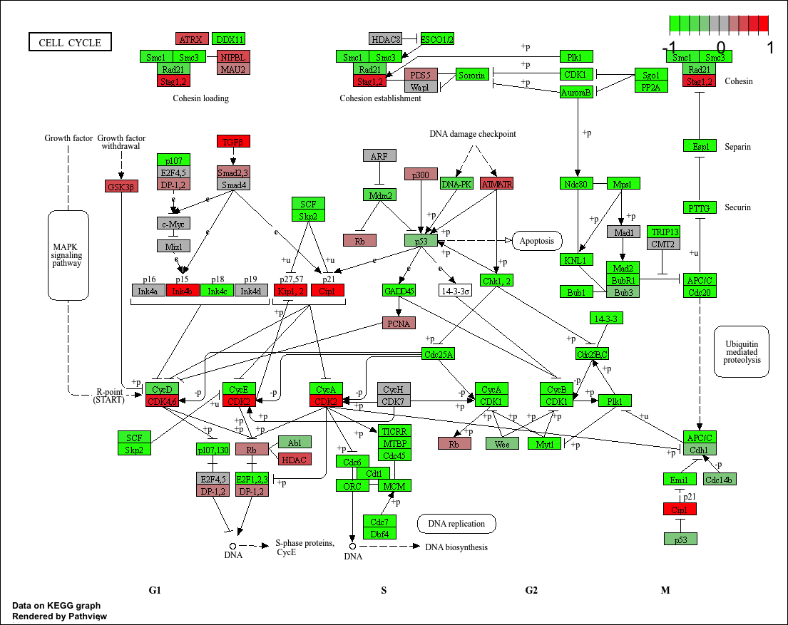
head(keggres$less)
                                         p.geomean stat.mean        p.val
hsa04110 Cell cycle                   8.995727e-06 -4.378644 8.995727e-06
hsa03030 DNA replication              9.424076e-05 -3.951803 9.424076e-05
hsa03013 RNA transport                1.375901e-03 -3.028500 1.375901e-03
hsa03440 Homologous recombination     3.066756e-03 -2.852899 3.066756e-03
hsa04114 Oocyte meiosis               3.784520e-03 -2.698128 3.784520e-03
hsa00010 Glycolysis / Gluconeogenesis 8.961413e-03 -2.405398 8.961413e-03
                                            q.val set.size         exp1
hsa04110 Cell cycle                   0.001448312      121 8.995727e-06
hsa03030 DNA replication              0.007586381       36 9.424076e-05
hsa03013 RNA transport                0.073840037      144 1.375901e-03
hsa03440 Homologous recombination     0.121861535       28 3.066756e-03
hsa04114 Oocyte meiosis               0.121861535      102 3.784520e-03
hsa00010 Glycolysis / Gluconeogenesis 0.212222694       53 8.961413e-03
pathview(gene.data=foldchanges, pathway.id="hsa04110")
'select()' returned 1:1 mapping between keys and columns

Info: Working in directory /Users/samfisher/Bimm143_Github/bimm143_github/class14

Info: Writing image file hsa04110.pathview.png
knitr::include_graphics("hsa04110.pathview.png")
# A different PDF based output of the same data
pathview(gene.data=foldchanges, pathway.id="hsa04110", kegg.native=FALSE)
'select()' returned 1:1 mapping between keys and columns

Warning: reconcile groups sharing member nodes!

     [,1] [,2]
[1,] "9"  "300"
[2,] "9"  "306"

Info: Working in directory /Users/samfisher/Bimm143_Github/bimm143_github/class14

Info: Writing image file hsa04110.pathview.pdf
## Focus on top 5 upregulated pathways here for demo purposes only
keggrespPathways <- rownames(keggres$greater)[1:5]

## Extract the 8 character long IDs part of each string
keggResids <- substr(keggrespPathways, start=1, stop=8)
keggResids
[1] "hsa04640" "hsa04630" "hsa00140" "hsa04142" "hsa04330"
pathview(gene.data=foldchanges, pathway.id=keggResids, species="hsa")
'select()' returned 1:1 mapping between keys and columns

Info: Working in directory /Users/samfisher/Bimm143_Github/bimm143_github/class14

Info: Writing image file hsa04640.pathview.png

'select()' returned 1:1 mapping between keys and columns

Info: Working in directory /Users/samfisher/Bimm143_Github/bimm143_github/class14

Info: Writing image file hsa04630.pathview.png

'select()' returned 1:1 mapping between keys and columns

Info: Working in directory /Users/samfisher/Bimm143_Github/bimm143_github/class14

Info: Writing image file hsa00140.pathview.png

'select()' returned 1:1 mapping between keys and columns

Info: Working in directory /Users/samfisher/Bimm143_Github/bimm143_github/class14

Info: Writing image file hsa04142.pathview.png

'select()' returned 1:1 mapping between keys and columns

Info: Working in directory /Users/samfisher/Bimm143_Github/bimm143_github/class14

Info: Writing image file hsa04330.pathview.png
knitr::include_graphics(paste0(keggResids, ".pathview.png"))
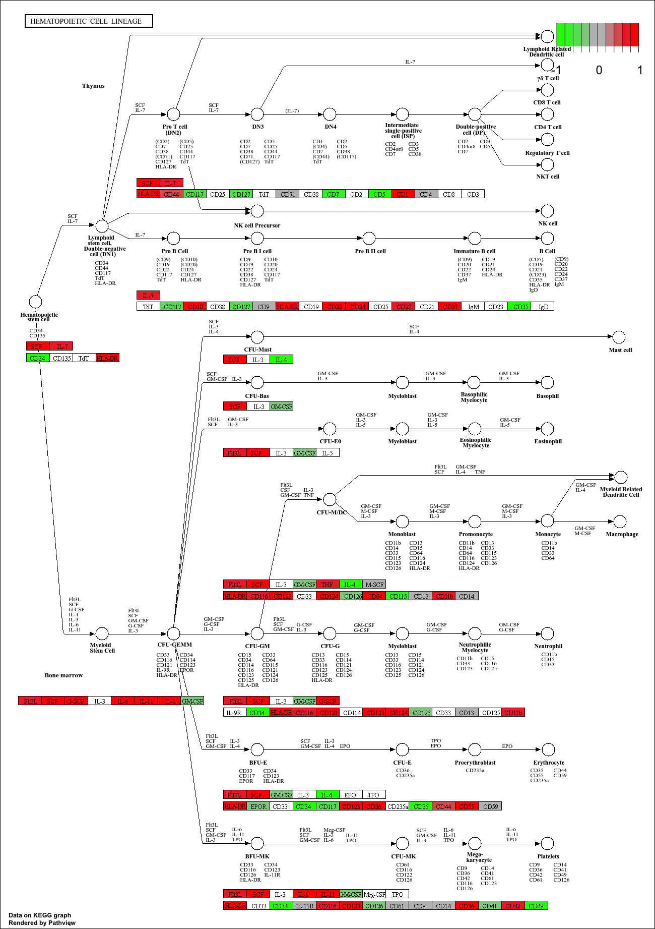
Q. Can you do the same procedure as above to plot the pathview figures for the top 5 down-regulated pathways?
Yes. The same procedure can be repeated using keggres$less instead of keggres$greater to get the top five down-regulated pathways. After getting the pathway IDs, they can be passed to the pathview() function to create the same corresponding pathway plots as above.
Section 3: Gene Ontology (GO)
data(go.sets.hs)
data(go.subs.hs)

# Focus on Biological Process subset of GO
gobpsets = go.sets.hs[go.subs.hs$BP]

gobpres = gage(foldchanges, gsets=gobpsets)

lapply(gobpres, head)
$greater
                                             p.geomean stat.mean        p.val
GO:0007156 homophilic cell adhesion       8.519724e-05  3.824205 8.519724e-05
GO:0002009 morphogenesis of an epithelium 1.396681e-04  3.653886 1.396681e-04
GO:0048729 tissue morphogenesis           1.432451e-04  3.643242 1.432451e-04
GO:0007610 behavior                       1.925222e-04  3.565432 1.925222e-04
GO:0060562 epithelial tube morphogenesis  5.932837e-04  3.261376 5.932837e-04
GO:0035295 tube development               5.953254e-04  3.253665 5.953254e-04
                                              q.val set.size         exp1
GO:0007156 homophilic cell adhesion       0.1951953      113 8.519724e-05
GO:0002009 morphogenesis of an epithelium 0.1951953      339 1.396681e-04
GO:0048729 tissue morphogenesis           0.1951953      424 1.432451e-04
GO:0007610 behavior                       0.1967577      426 1.925222e-04
GO:0060562 epithelial tube morphogenesis  0.3565320      257 5.932837e-04
GO:0035295 tube development               0.3565320      391 5.953254e-04

$less
                                            p.geomean stat.mean        p.val
GO:0048285 organelle fission             1.536227e-15 -8.063910 1.536227e-15
GO:0000280 nuclear division              4.286961e-15 -7.939217 4.286961e-15
GO:0007067 mitosis                       4.286961e-15 -7.939217 4.286961e-15
GO:0000087 M phase of mitotic cell cycle 1.169934e-14 -7.797496 1.169934e-14
GO:0007059 chromosome segregation        2.028624e-11 -6.878340 2.028624e-11
GO:0000236 mitotic prometaphase          1.729553e-10 -6.695966 1.729553e-10
                                                q.val set.size         exp1
GO:0048285 organelle fission             5.841698e-12      376 1.536227e-15
GO:0000280 nuclear division              5.841698e-12      352 4.286961e-15
GO:0007067 mitosis                       5.841698e-12      352 4.286961e-15
GO:0000087 M phase of mitotic cell cycle 1.195672e-11      362 1.169934e-14
GO:0007059 chromosome segregation        1.658603e-08      142 2.028624e-11
GO:0000236 mitotic prometaphase          1.178402e-07       84 1.729553e-10

$stats
                                          stat.mean     exp1
GO:0007156 homophilic cell adhesion        3.824205 3.824205
GO:0002009 morphogenesis of an epithelium  3.653886 3.653886
GO:0048729 tissue morphogenesis            3.643242 3.643242
GO:0007610 behavior                        3.565432 3.565432
GO:0060562 epithelial tube morphogenesis   3.261376 3.261376
GO:0035295 tube development                3.253665 3.253665
Section 4: Reactome Analysis
sig_genes <- res[res$padj <= 0.05 & !is.na(res$padj), "symbol"]
print(paste("Total number of significant genes:", length(sig_genes)))
[1] "Total number of significant genes: 8147"
write.table(sig_genes,
            file="significant_genes.txt",
            row.names=FALSE,
            col.names=FALSE,
            quote=FALSE)
Q: What pathway has the most significant “Entities p-value”? Do the most significant pathways listed match your previous KEGG results? What factors could cause differences between the two methods?
The pathway with the most significant “Entities p-value” is Cell Cycle, Mitotic. The top Reactome pathways match well with our previous KEGG results. Minor differences may arise due to differences in pathway databases, gene set definitions, statistical models, and multiple testing correction procedures.